Predicting Stock Prices from the DJIA
Daniela De la Parra
Machine Learning Engineer Nanodegree: Capstone Proposal
June 2020
Project Overview
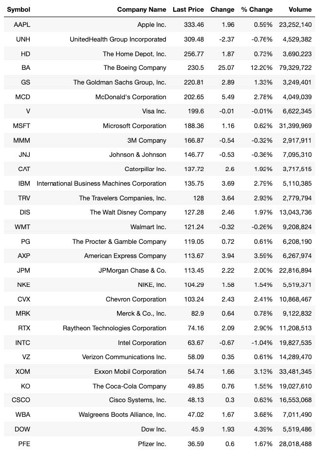
The Dow Jones Industrial Average (DJIA) is a stock market index that tracks the performance of 30 large public companies traded in the New York Stock Exchange and NASDAQ. The DJIA is one of the commonly followed stock indices, and it is meant to reflect the overall health of the U.S. economy. The stocks in this index are thought to be well-established and stable, relative to other stocks. However, prior research has found that these companies are still affected by large shocks, including financial crashes, monetary policies, elections, and wars [1]. The table below shows the price, change, % change, and volume of the 30 companies in the DJIA, as of June 8, 2020 [2]. As we can see, the index includes some of the largest, well-known companies.
Given the popularity of machine learning algorithms and their powerful predictive ability, prior research has tried to implement these techniques to analyze stock market data and predict stock prices [3]. Some have constructed sophisticated trading algorithms based on technical indicators, which are mathematical indicators based on a stock’s patterns in price, volume, etc [4]. Others have used the textual content of managerial disclosures [5] or stochastic discount factors [6]. In this project, I will use the time series of stock prices of the components of the DJIA to see how well a machine learning model can predict their prices.
Problem Statement
For this project, my objective is to build a stock price predictor that takes daily stock prices of the DIJA components over a certain date range as input, and outputs projected estimates of the closing price for given query dates.
My implementation consists of two components:
- A training interface that accepts a data range (start_date, end_date) and a list of ticker symbols from the DJIA (e.g. PFE, AAPL), and builds a model of stock behavior.
- An estimation stage that accepts a list of dates and a list of ticker symbols from the DJIA, and outputs the predicted stock prices for each of those stocks on the given dates. The query dates passed in must be after the training date range, and ticker symbols must be a subset of the ones trained on.
Metrics
I use a moving average model as my benchmark, and I evaluate this and the DeepAR models from Amazon SageMaker by comparing their predictions to a known target. I calculate the root-mean-square error (RMSE) and compare the performance of the models. I decided to use this metrics score because it is well suited for regression-type predictions rather than classification. That is, even if the predictions are not perfectly equal to the true targets, the closer they are to the truth the better the performance of the model.
I also plot the results for each company for ease of visualization. The data for the target will come from my test sample, the true stock prices of companies. I create a plot with 90 or 80% confidence intervals to see how well the models did.
Data Exploration
The dataset for this project consists of daily stock prices of DJIA components from January 1, 2017 to May 31, 2020. I use the full years 2017, 2018, and 2019 to train the model, and the data for 2020 to test it.
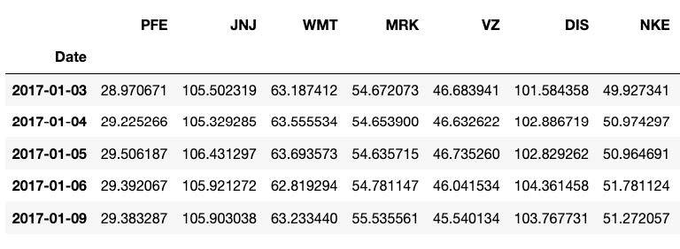
I use the package yfinance to download stock data from Yahoo Finance. To install this package, run pip install yfinance in the terminal. The data files are included in the folder data/. I am only interested in predicting the closing price of the day, so I only keep the column “Close” and the column “Date” to be used as the index of the pandas dataframes I construct. Here is what the data looks like for the first seven companies and their first six days of data:
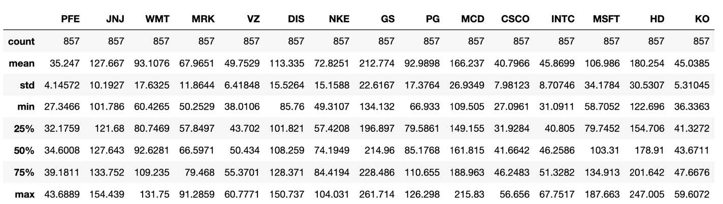
My data includes 857 rows representing one trading day each. Stock exchanges are usually closed on weekends and during holidays. A tabulation of the years in my data shows that I have 251 days in 2017, 251 in 2018, 252 in 2019, and 103 in 2020.
Here is a description of the closing price of each company:
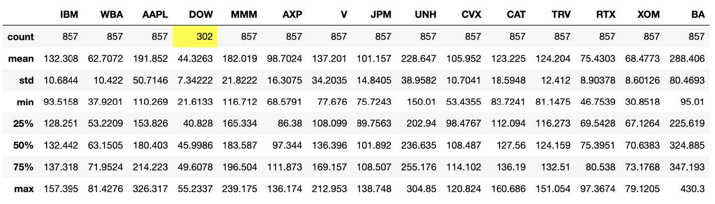
Notice that Dow Inc., with ticker DOW, only has 302 rows of data. The reason is that this company was created in early 2019, when DowDuPont Inc. split into three companies. One of them, Dow Inc., ended up replacing DowDuPont Inc. in the DJIA index [7]. In fact, once we look into DOW’s time series, we see that it indeed starts in March of 2019:
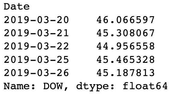
Given that training the model with only 302 might result in less accurate predictions, I decided to drop this company from my analysis. I thus have only 29 companies in my dataset.
Exploratory Visualization
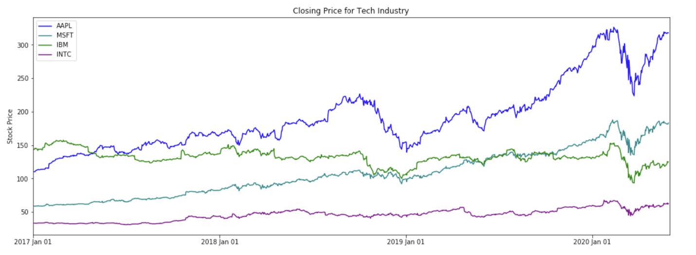
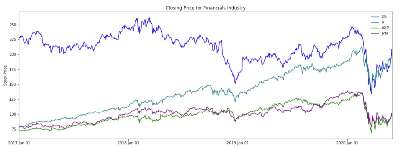
The DJIA data not only varies in terms of the volume and price level of its stocks, but it also varies in industry composition. As an illustration, we can review the stock behavior of stocks in the tech industry and financial stocks.
To observe the stock price patterns of all the components of the DJIA, we can create subplots that show the trend in each company individually:
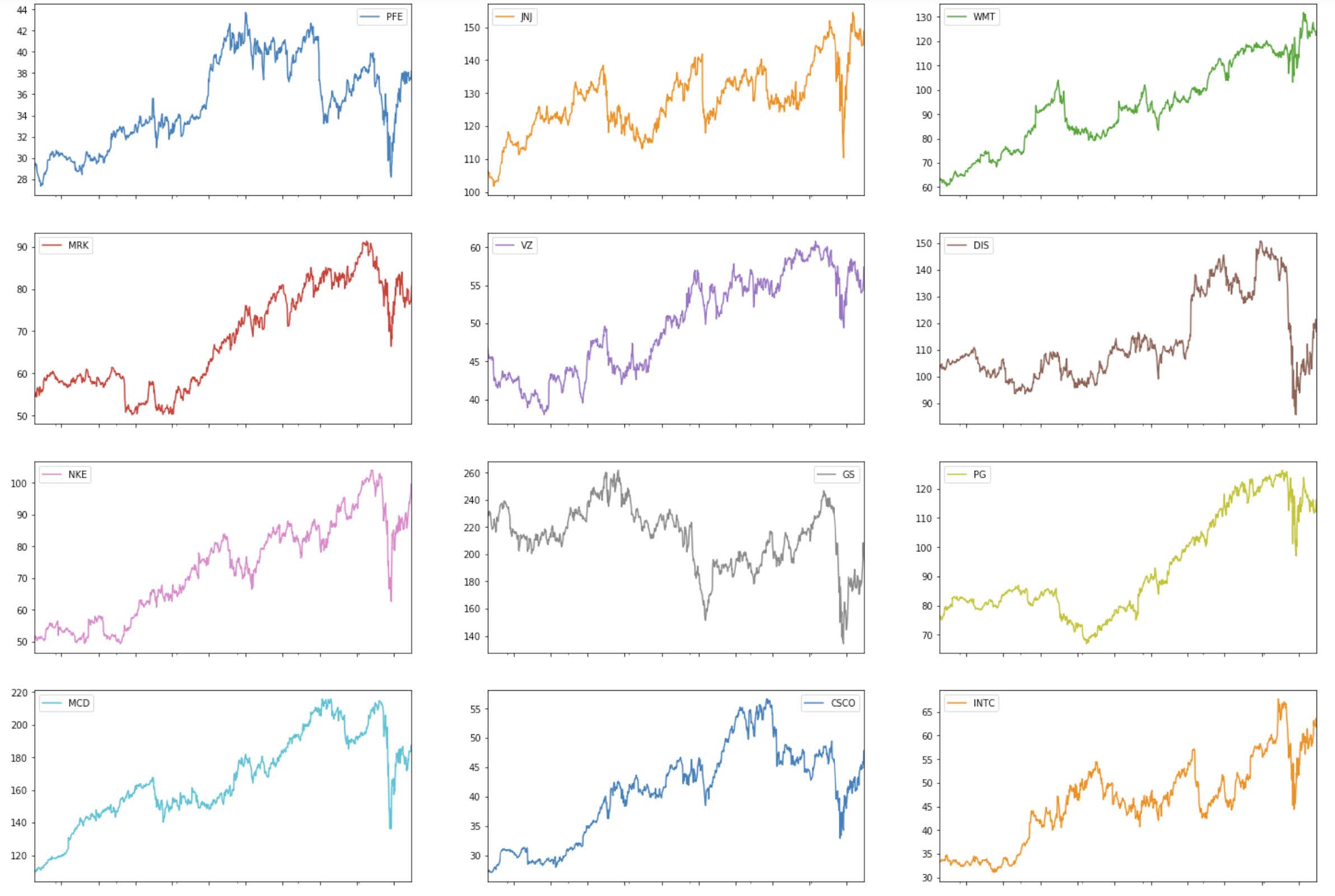
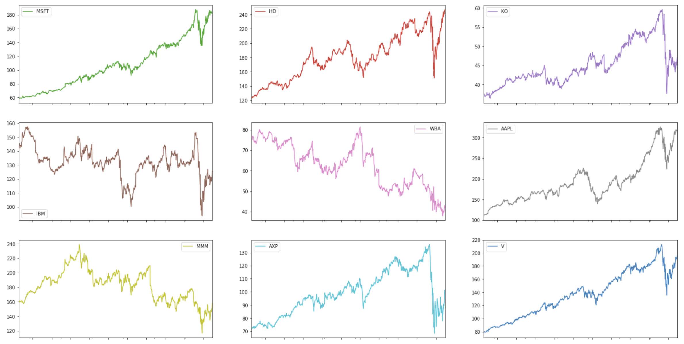
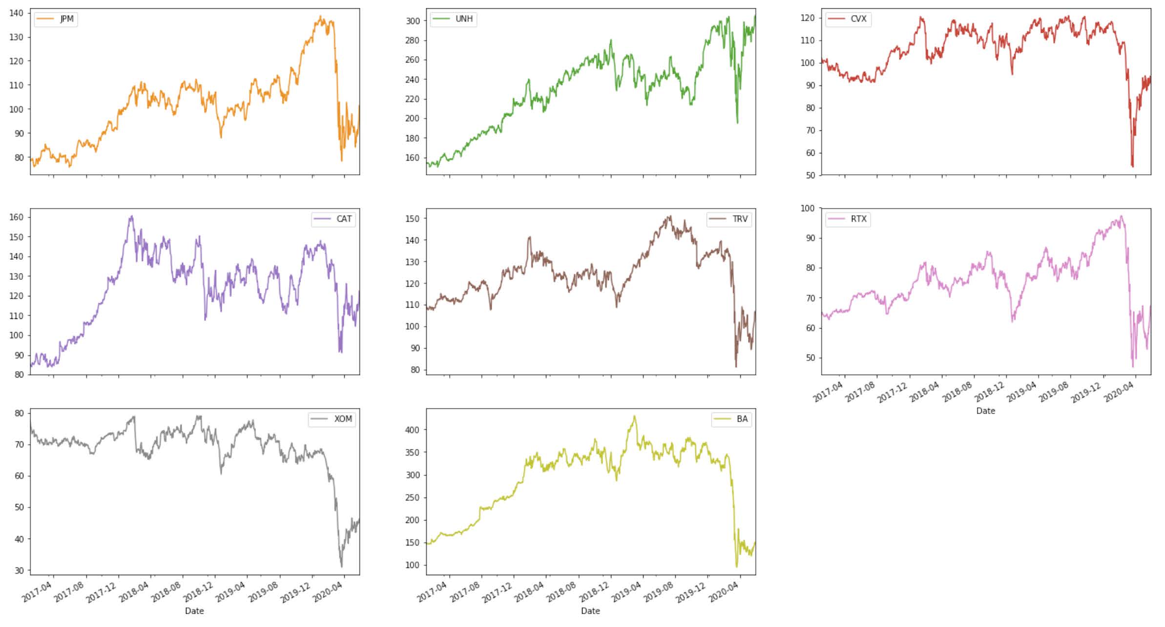
Notice that the majority of the stocks show an increasing pattern during 2017, 2018, and 2019, with a sharp increase at the beginning of 2020, likely due to the coronavirus pandemic. However, there are some stocks that show an overall declining trend (e.g. WBA), or consistent volatility (e.g. GS, IBM, XOM).
Algorithms and Techniques
To solve my problem, I use the first three years of data (from 2017-01-01 to 2019-12-31) to train and validate the model, and the rest of the data (from 2020-01-01 to 2020-05-31) to test the predictions. I use the SageMaker platform to instantiate and train a DeepAR estimator. After deploying the model and creating a predictor, I evaluate my model’s predictive ability to assure its accuracy score is reasonable. I also assess my model by making predictions on tickers and dates after my training period. Lastly, I compare the performance of my DeepAR model to the benchmark performance, which comes from a moving average model.
Benchmark
As a benchmark, I use an ARIMA(0,1,10) model, which is a moving average model based on the last 10 days of stock data. Moving averages, and ARIMA models in general, are common tools used in technical analysis to smooth out prices and create forecasts. The equation for a q-th order integrated moving average model with constant (ARIMA(0,1,p)) is [8]:
\[y_t = \mu + y_{t-1} + \epsilon_t - \phi_1 \epsilon_{t-1} - \phi_2 \epsilon_{t-2} - ... - \phi_p \epsilon_{t-p}\]Data Preprocessing
The input that DeepAR takes must be time series, so first I need to convert my data into time series objects. Each company’s stock price data is converted into a time series. The function that I write sets 2017-01-03 as the starting date (the first trading day of 2017) and 2019-12-31 as the ending date for each time series. Given that there are only 251 or 252 days in each year, each time series has 754 observations [9].
Here is the time series of company with ticker “PFE” to illustrate what my time series data looks like:
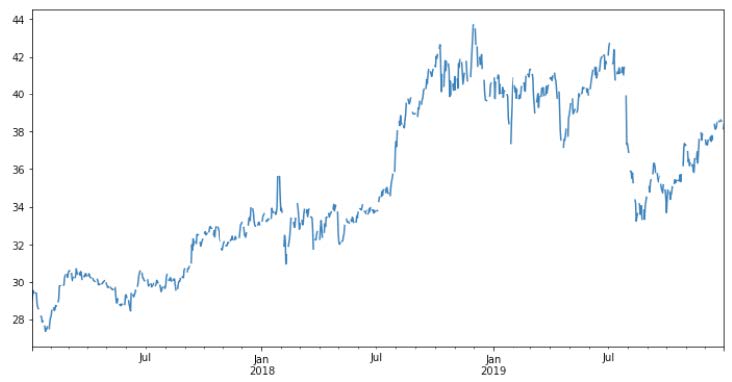
Notice that the line is not continuous, which reflects the fact that the stock price value for weekends and holidays is “NaN,” given that the stock market is closed.
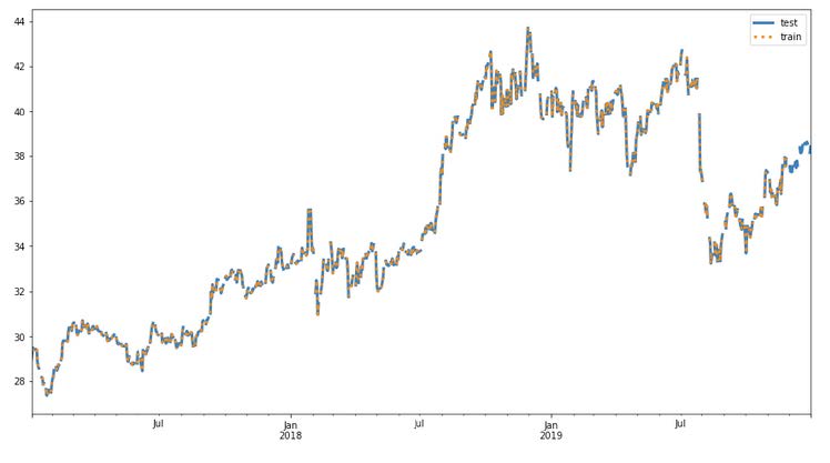
I next split my data into train and test samples for each time series. I do this using a prediction length of 30 days. I decided to only try to predict 30 days in advance because predicting stock prices is already extremely hard, so choosing a wider window would pose a substantial challenge to any model.
Here is what the train and test samples of the company “PFE” look in a graph:
Next, I need to encode each time series into a json object to pass it to the DeepAR estimator. I also need to save the files locally before uploading them to S3. The DeepAR documentation explains that I must encode missing values in the target as strings “NaN”, so I make sure that my function to convert my data into json also cleans these missing values.
Once I convert my data into json objects and save the files locally, I upload them to S3. Here are the directories where my data is saved
Training data is stored in: s3://sagemaker-us-east-2-551451770570/deeparstock-
prices/train/train.json
Test data is stored in: s3://sagemaker-us-east-2-551451770570/deepar-stockprices/
test/test.json
Implementation
I first instantiate a DeepAR estimator using SageMaker’s ‘forecasting-deepar’ image_name. I set the frequency of my data to daily (‘D’) and the context_length to 30, which means that the model will look back to 30 days of data in order to make a prediction. I use the following hyperparameters:
- epochs: 50
- time_freq: ‘D’
- prediction_length: 30
- context_length: 30
- num_cells: 50
- num_layers: 2
- mini_batch_size: 128
- learning_rate: 0.001
- early_stopping_patience: 10
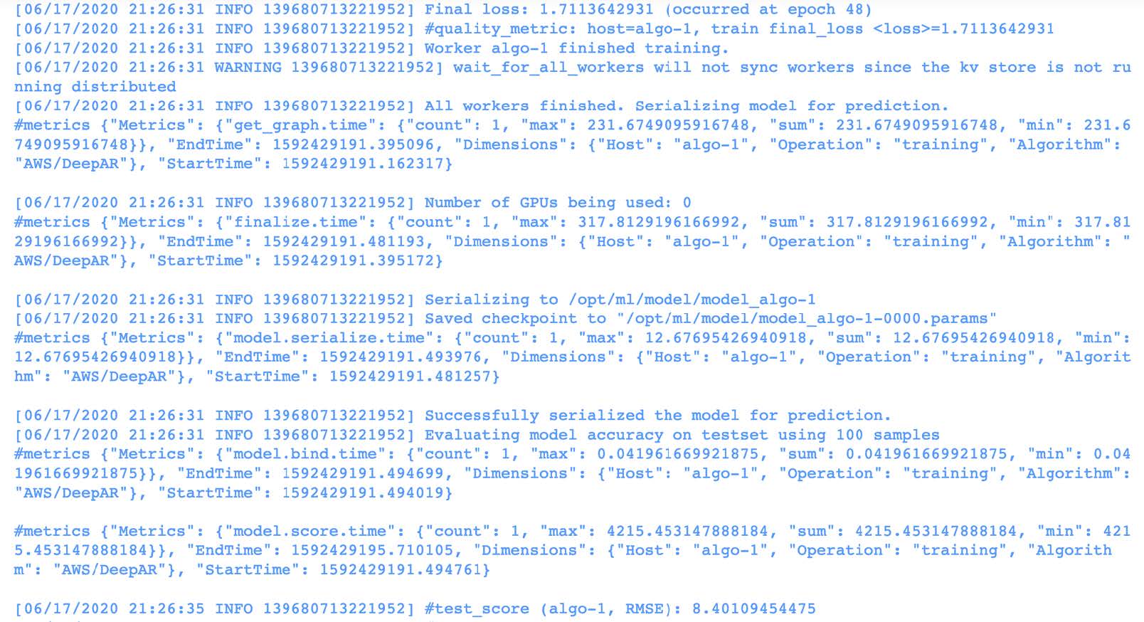
Next, I launched a training job that took a little more than 6 minutes to train. Based on the output from the training job, the model achieved its higher performance during epoch 48, with a final loss of 1.7113642931 and a test RMSE score of 8.4:
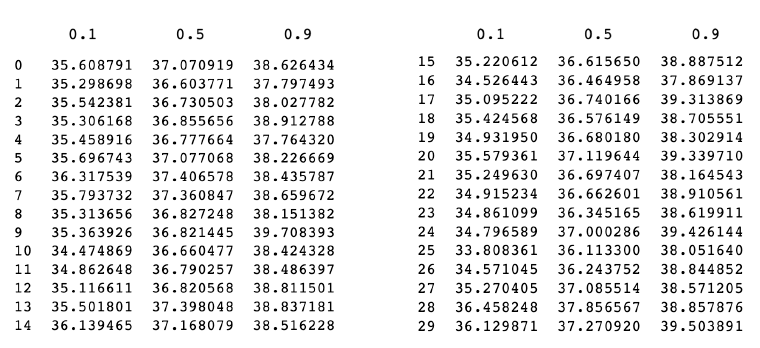
I then create a predictor object to generate predictions of the 20%, 50%, and 90% quantiles. I converted my time series into json objects in order to pass them to the predictor object, and then decode the predictions obtained. Here are the 30-day predictions for company “PFE”:
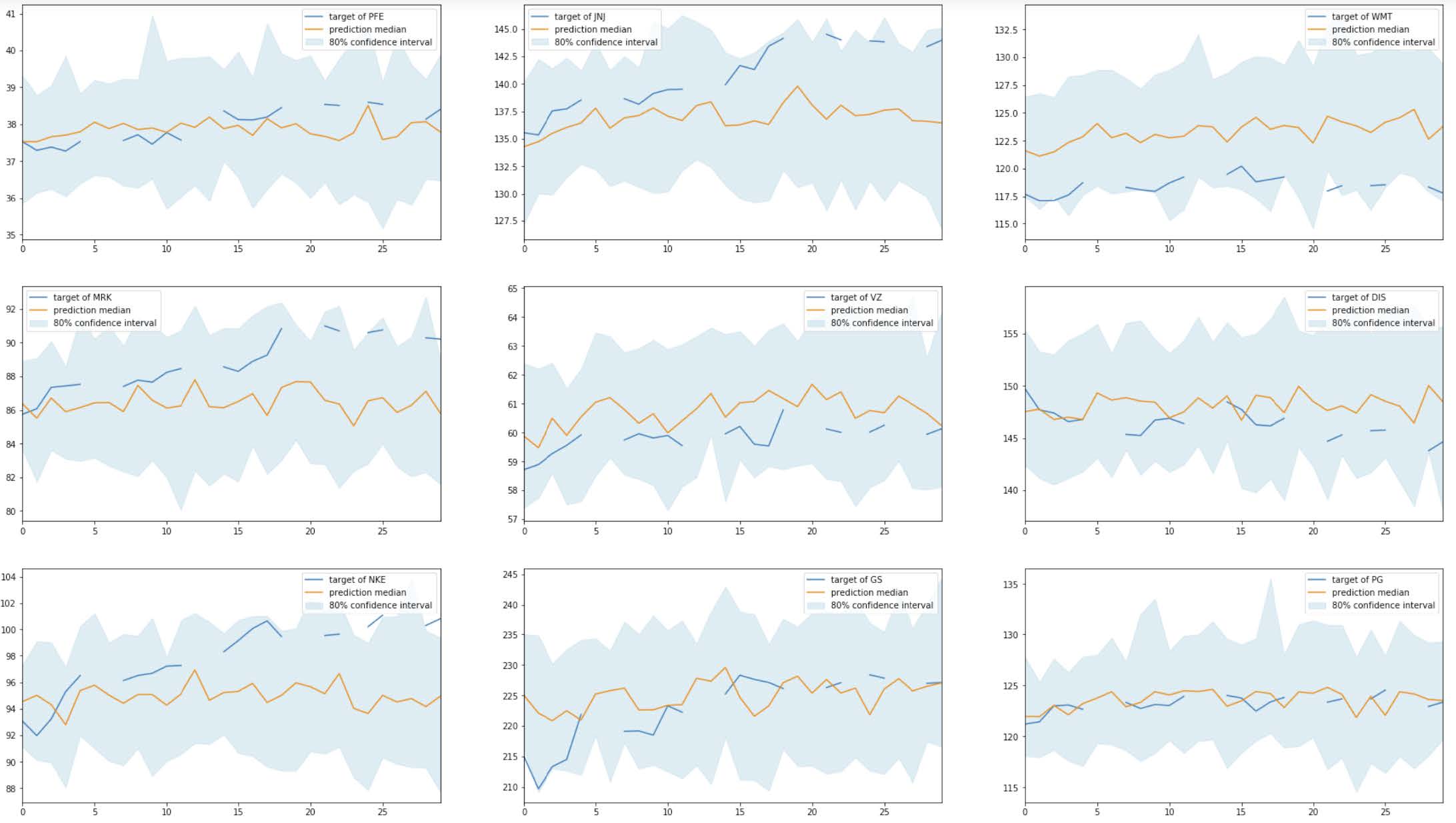
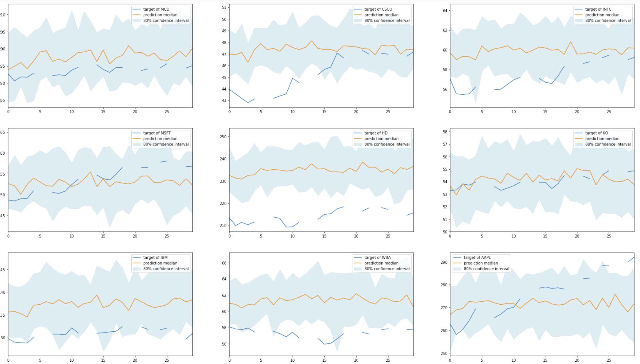
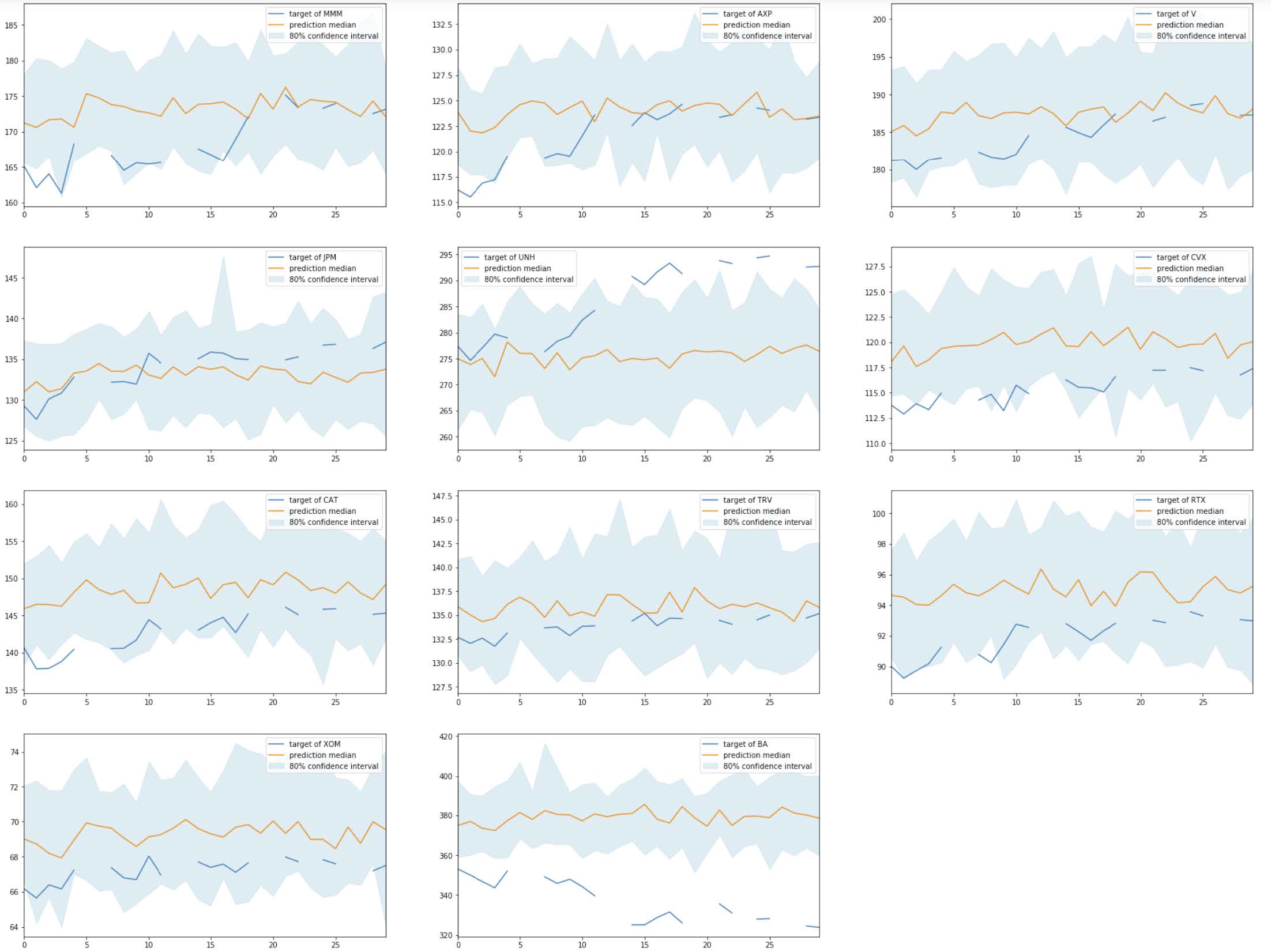
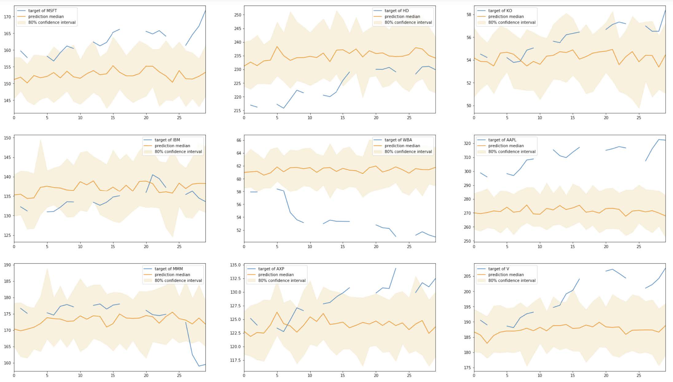
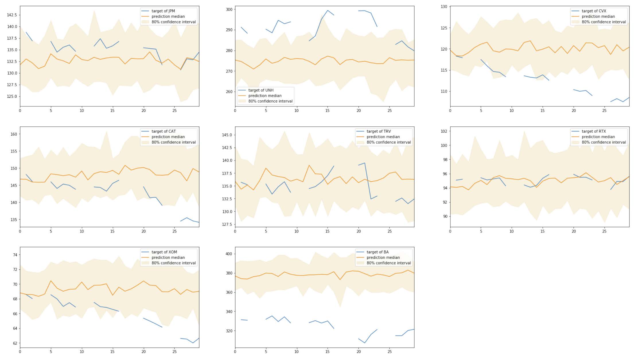
I create subplots to visualize the predictions vs. the true stock prices of each companies. The yellow areas indicate the 80% quantiles.
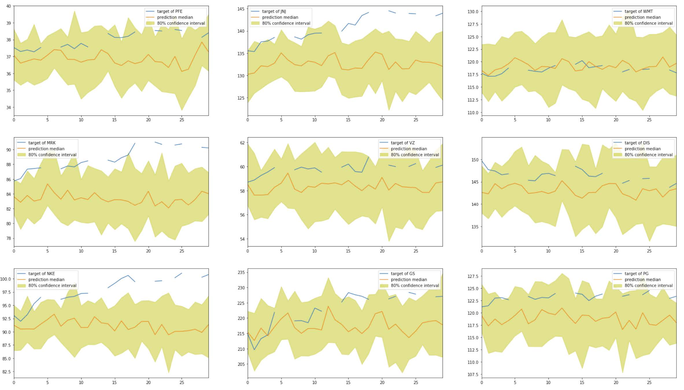
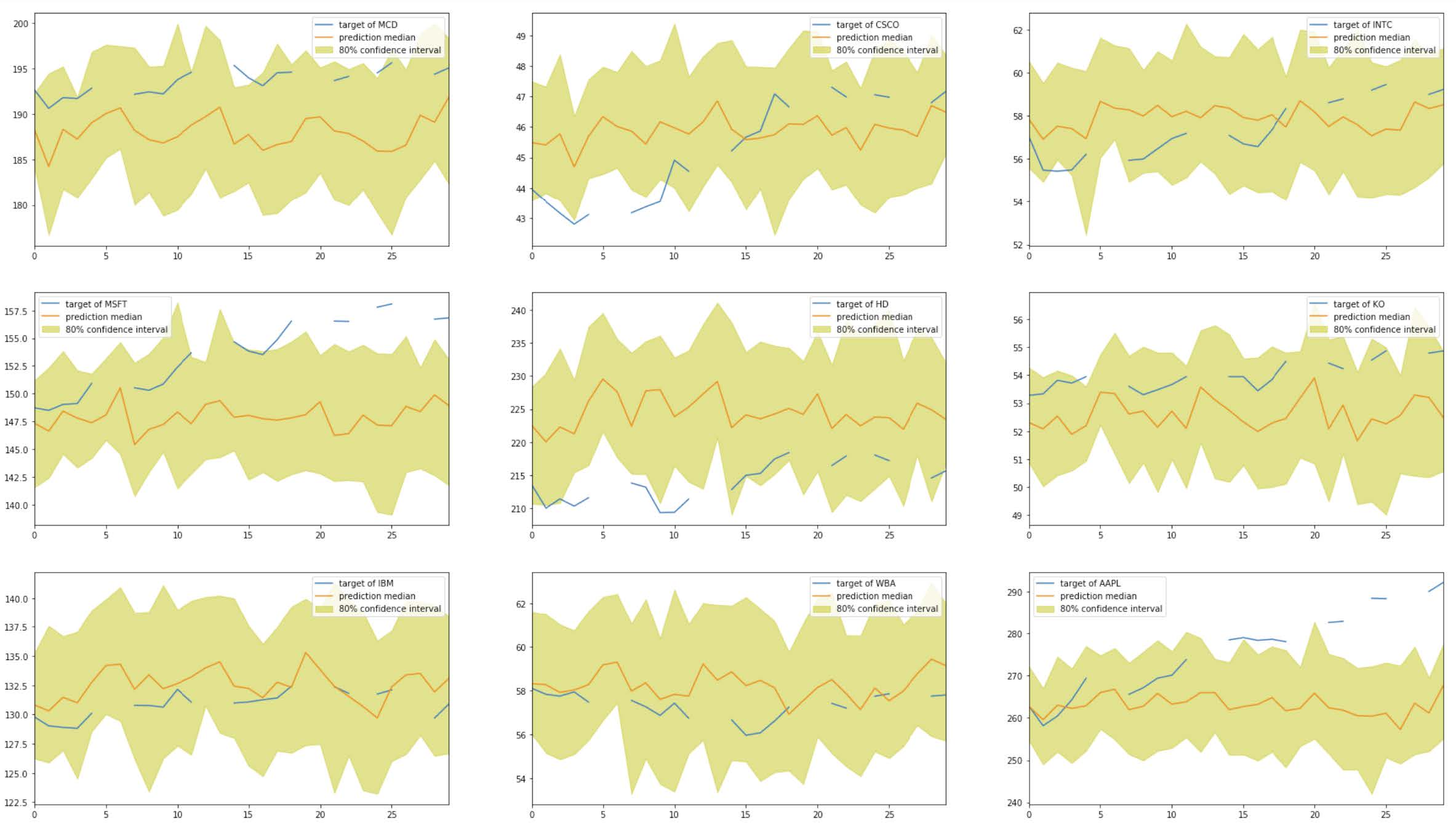
Based on the graphs, we can see that the model made reasonable predictions only for a few companies (e.g., KO, WBA, TRV). For many time series, the model made predictions very far from the true stock prices (e.g., JNJ, MRK, NKE, APPL, UNH, BA).
For comparison purposes, I calculate the root-mean-square error (RMSE) for these results on the test set. The RMSE score is 8.212, which seems high.
Refinement
Given that the model I trained did not produce reasonable predictions for many companies, in this section I attempt to improve the model’s predictive ability by automatically tuning its hyperparameters. The DeepAR documentation shows the following options for hyperparameter tuning:
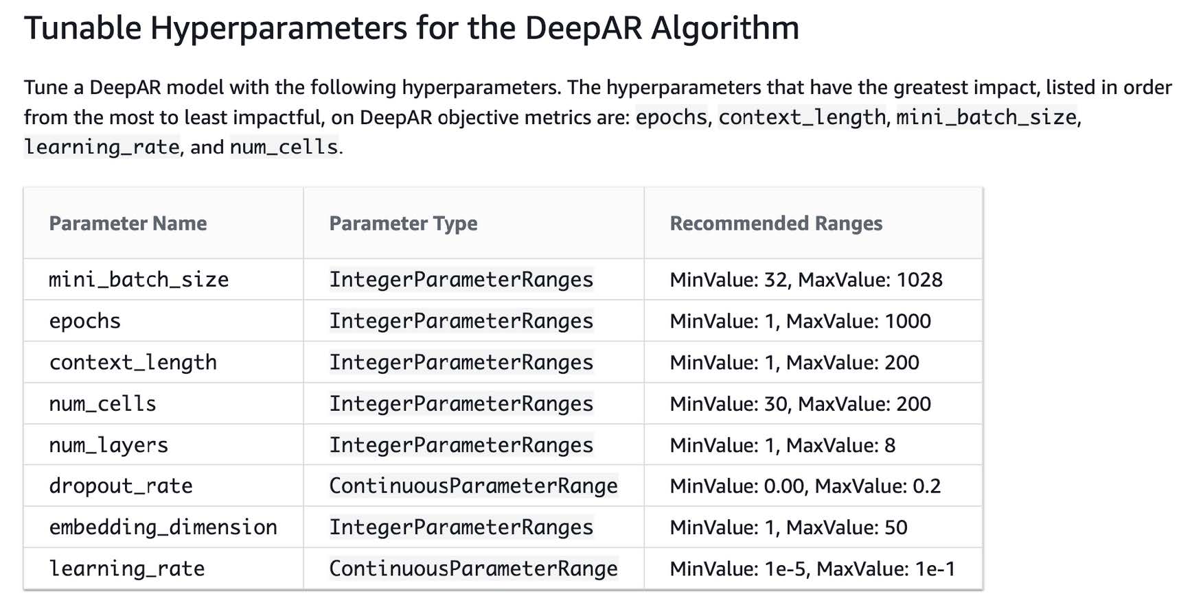
After instantiating a new estimator and setting default hyperparameters, I utilize SageMaker’s HyperparameterTuner to choose ranges for the parameters I want to tune. Specifically, I choose the following ranges:
num_cells : IntegerParameter(50, 70)
num_layers : IntegerParameter(2, 6)
learning_rate : ContinuousParameter(1e-5, 1e-2)
After the job is finished, I select the best training job. According to the training output, the following is the best configuration:
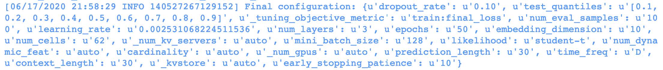
Out of the ranges of hyperparameters that I input in the hyperparameter_tuner, this is the configuration that achieved the highest performance:
learning_rate : '0.002531068224511536'
num_layers : '3'
num_cells : '62'
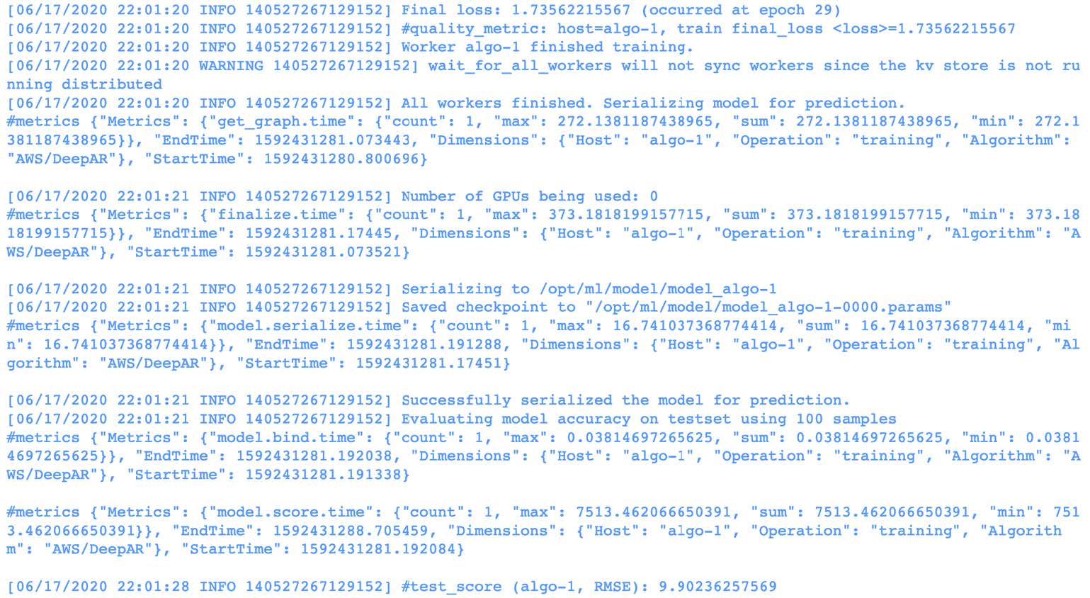
The model achieved its higher performance during epoch 29, with a final loss of 1.73562215567 and a test RMSE score of 9.9:
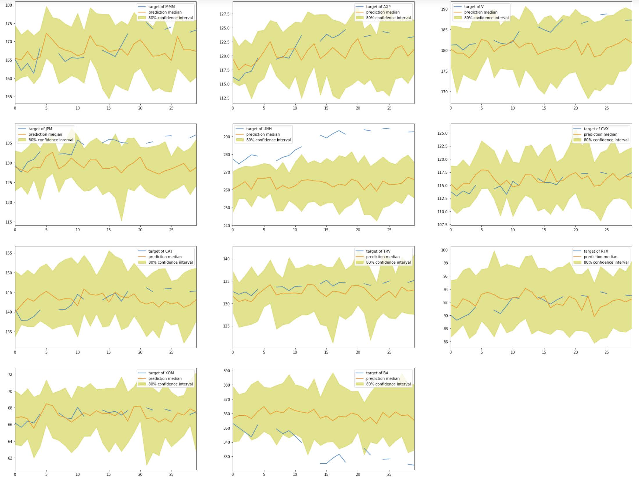
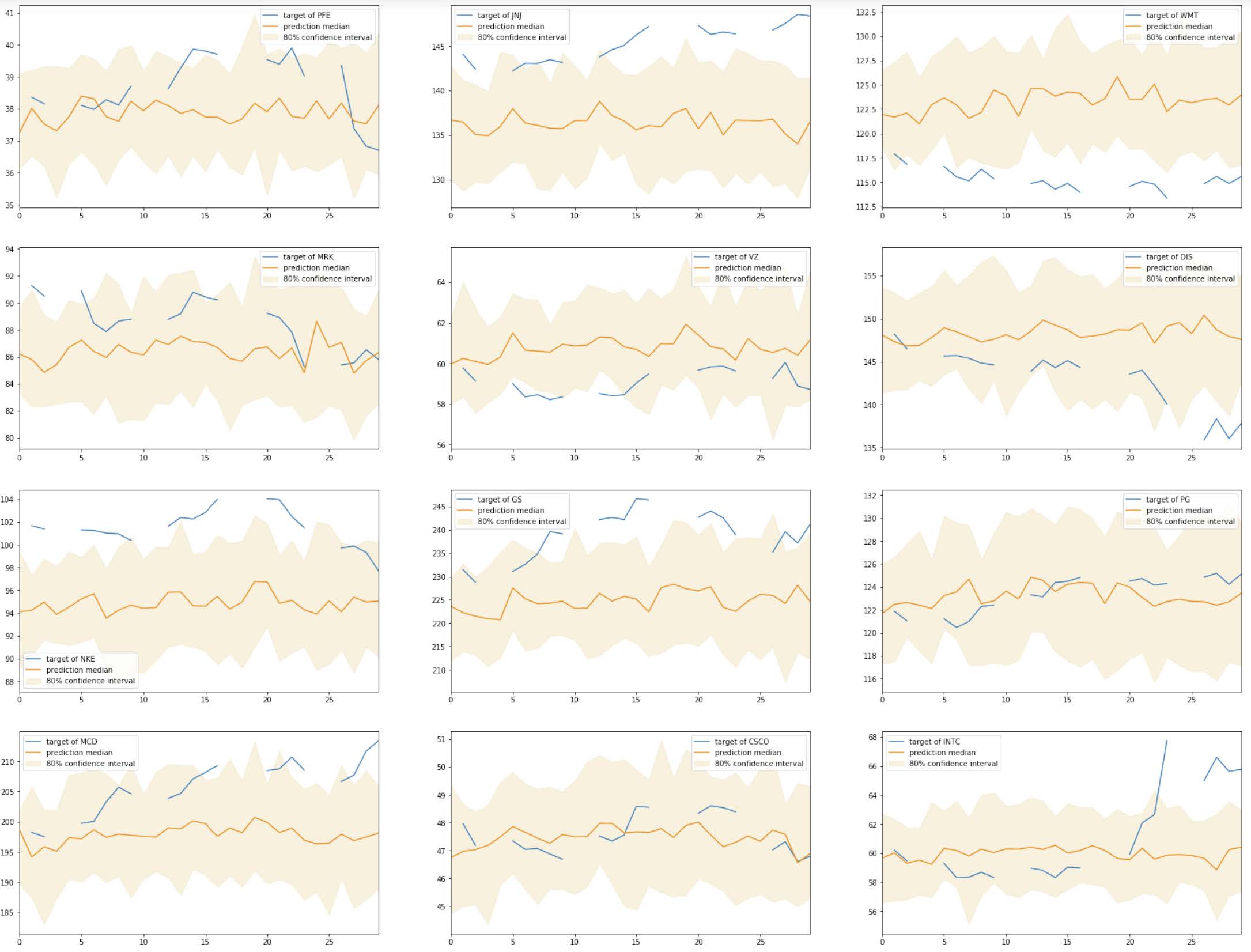
I create a predictor based on this hypertuned model, and I evaluate the predictions for each company, compared to the true stock prices. Below are the plots of the results:
Based on the graphs, it does not look like the model improved much using the new configuration of hyperparameters. In fact, the RMSE of this refined model is 10.035, which is higher than the original model. This is surprising because I passed the same default parameters as the ones I used for the original model. The only difference is that the refined model was automatically tuned using the ranges of hyperparameters I passed.
Model Evaluation and Validation
I evaluate and validate my model using the data in 2020 that the model has not seen. I first input each company’s time series into json and send it to the predictor. After decoding the predictions, I compare them directly with the true stock prices of 2020.
The results are plotted against 80% confidence intervals and are shown below:
Not surprisingly, these predictions are worse than in the training set. The RMSE of the results is 14.634. These results reflect the challenge in predicting stock prices using only their past price as guidance. It also sheds light into the difficulty in finding appropriate hyperparameters. Perhaps training the model for more epochs and using mode layers could improve the results.
Justification
I compare my final results to my benchmark, which is an ARIMA(0,1,10) model, or integrated moving average, that uses the last 10 days of stock data. As I mentioned earlier, this is an appropriate model because moving averages are common tools used in technical analysis make predictions [10].
The ARIMA model takes last 10 days of data and makes a prediction, which I then append to the history of data and use to make the following day’s prediction.
The model trained for about 13 minutes, and it reached a performance of RMSE = 1.703. This is the best performing model, according to this metric. To illustrate the results, the predictions are plotted against the targets for each company:
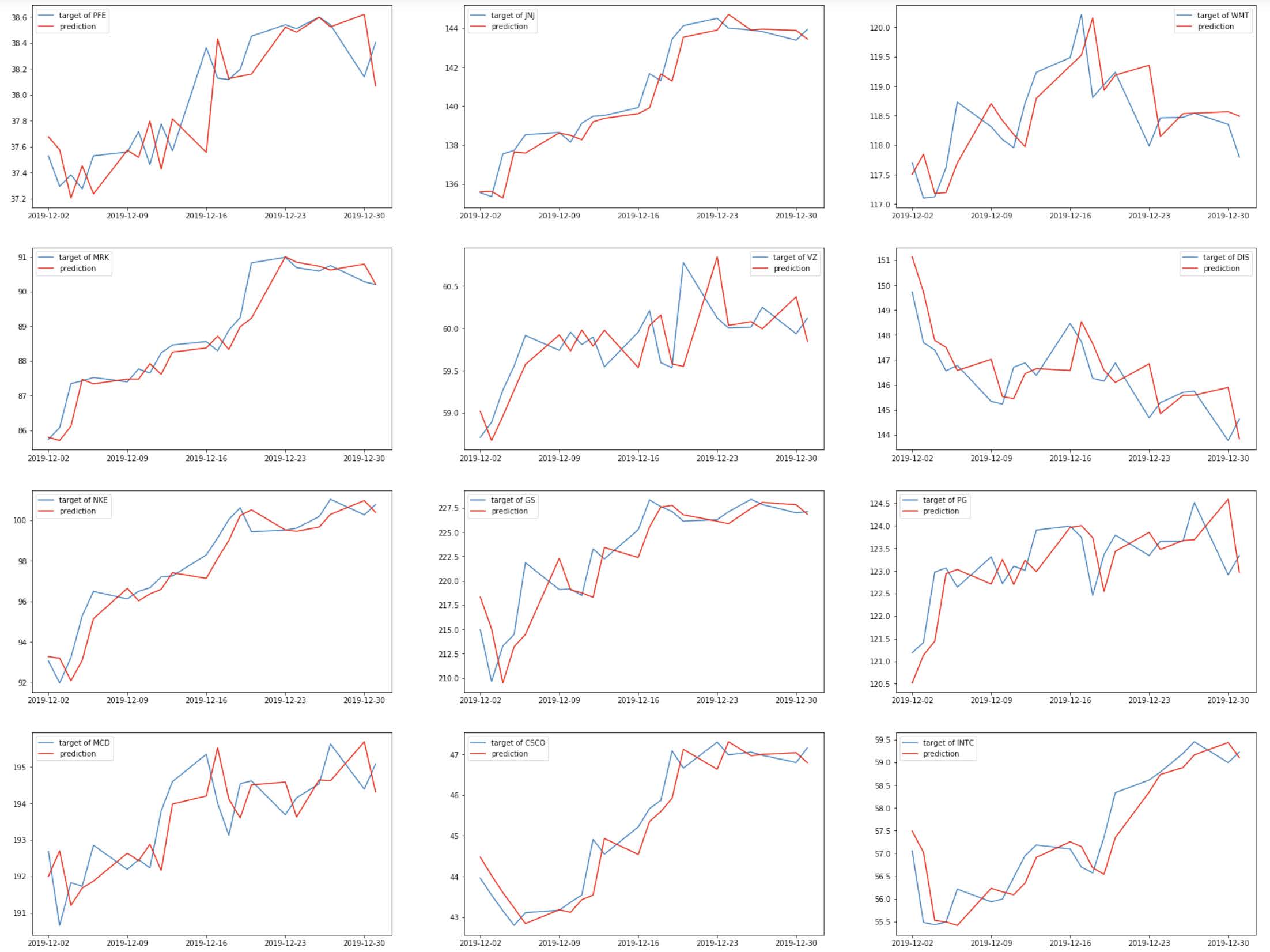
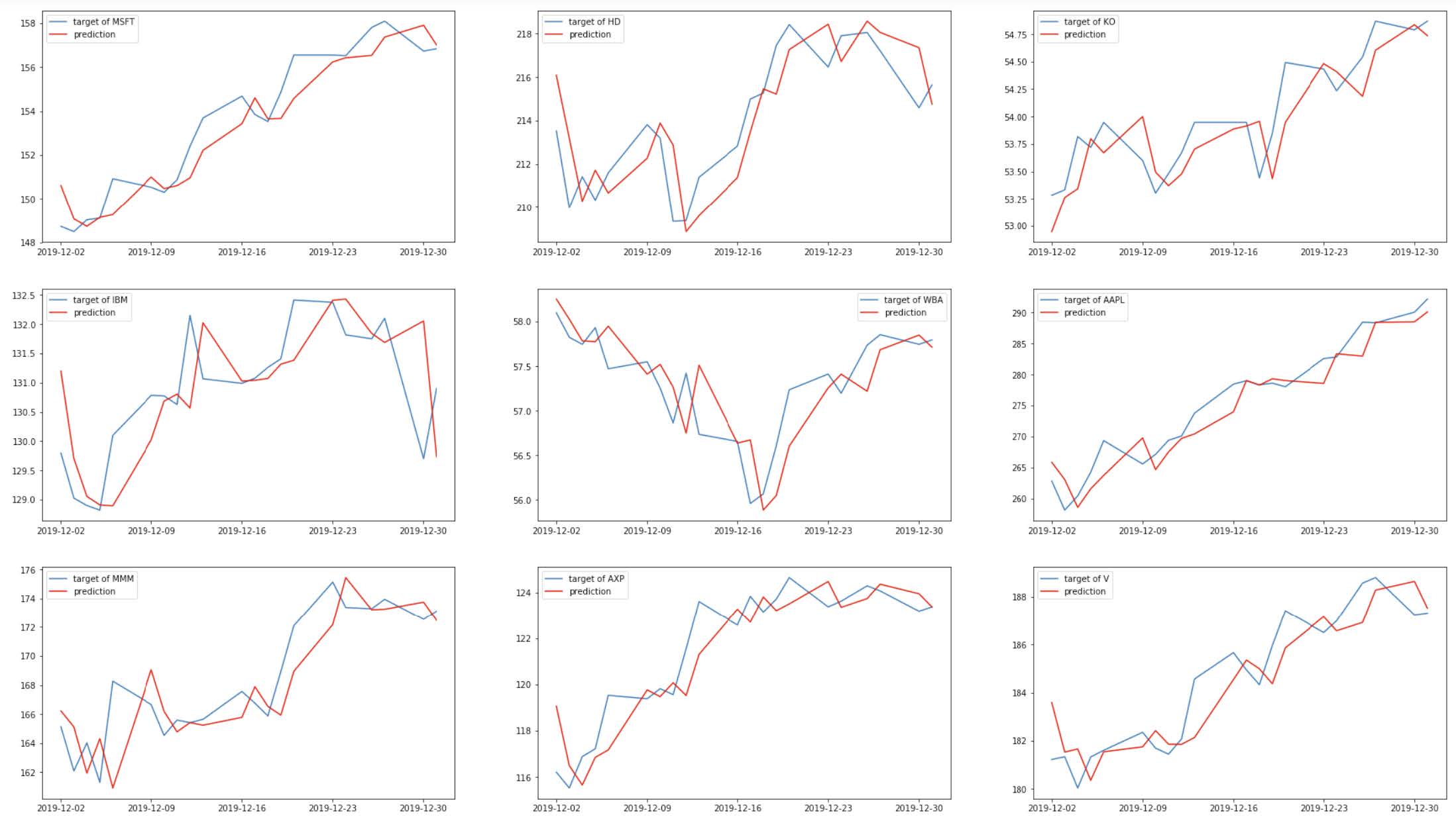
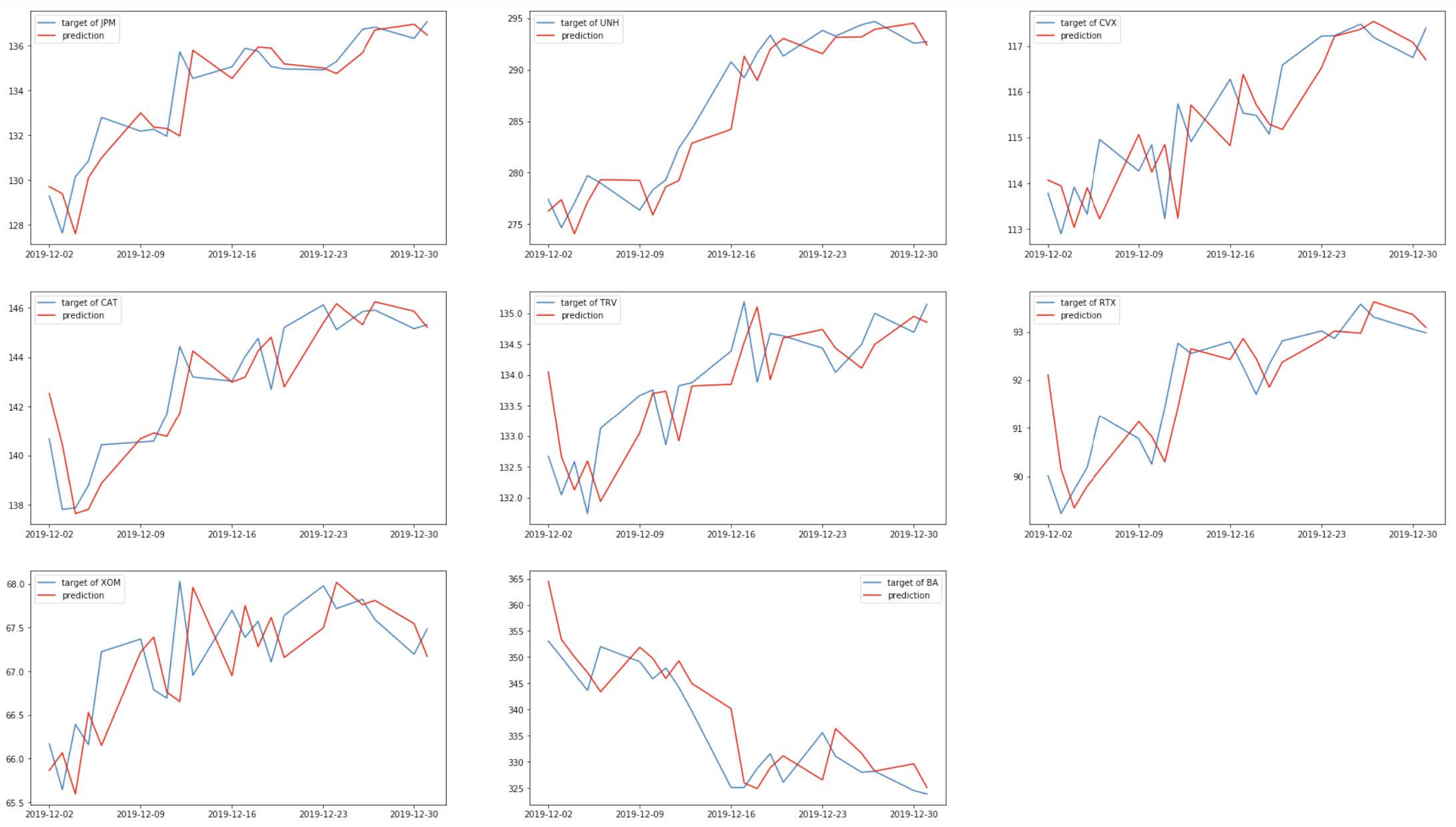
It seems like the predictions of this model more closely follow the true stock prices. Intuitively, recent price movements are an indicator of where the market is heading and how investors are interpreting information, although their predictive ability is far from perfect.
Conclusion
In this project, I analyzed stock market data from the DJIA components. Specifically, I constructed machine learning models to try to predict stock prices 30 days in advance. An exploration analysis revealed that the stock prices of these companies are often volatile, as expected from stock market data. In order to solve the prediction problem, I implemented a DeepAR model that was trained using the first three years of data of my time series. The model reached its best performance during epoch 48 and reached an RMSE score of 8.4. Based on this score and on a visual examination of the plotted predictions against the true stock prices, I decided to attempt to improve the model’s prediction by instantiating and training a refined model that used automatic hyperparameter tuning. I selected ranges for the number of layers, the number of cells per layer, and the learning rate. The predictive ability of the refined model, however, did not seem to improve much from the original model. The highest performance was attained during epoch 29, with an RMSE score of 9.9.
I also evaluated the model in the test set, using data from 2020, which the model had never seen. In this test data, the model reached an RMSE score of 14.6, which shows that it is harder to predict data on the test sample than the train sample. Lastly, I compared the results to an ARIMA(0,1,10) model based on the last 10 days of data. This benchmark model actually had the best performance in terms of RMSE, reaching a score of 1.7. The results from my analysis shed light into the challenge of predicting stock prices when we only use past stock prices information. Sophisticated traders and professional investors use not only stock prices, but also an extensive amount of data that includes corporate disclosures, industry trends, and macroeconomic indicators. I believe that my model would substantially benefit from incorporating other types of information, such as accounting data from companies’ financial statements.
References
- Charles, A., & Darné, O. (2014). Large shocks in the volatility of the Dow Jones Industrial Average index: 1928–2013. Journal of Banking & Finance, 43, 188-199.
- https://finance.yahoo.com/quote/%5EDJI/components?p=%5EDJI, accessed on 2020-06-08.
- Shen, S., Jiang, H., & Zhang, T. (2012). Stock market forecasting using machine learning algorithms. Department of Electrical Engineering, Stanford University, Stanford, CA, 1-5.
- Dash, R., & Dash, P. K. (2016). A hybrid stock trading framework integrating technical analysis with machine learning techniques. The Journal of Finance and Data Science, 2(1), 42-57.
- Jiang, F., Lee, J., Martin, X., & Zhou, G. (2019). Manager sentiment and stock returns. Journal of Financial Economics, 132(1), 126-149.
- Kozak, S., Nagel, S., & Santosh, S. (2020). Shrinking the cross-section. Journal of Financial Economics, 135(2), 271-292
- https://www.reuters.com/article/us-usa-stocks-dowdupont/dow-jones-industrial-average-adds-dow-inc-removesdowdupont-idUSKCN1R72TP
- https://people.duke.edu/~rnau/411arim.htm#ses
- I learned to implement this model based on the code from my lessons during the Nannodegree program. Here are the links to the files I looked at: https://github.com/udacity/sagemaker-deployment/blob/master/Tutorials/Boston%20Housing%20-%20XGBoost%20(Hyperparameter%20Tuning)%20-%20High%20Level.ipynb, and https://github.com/udacity/ML_SageMaker_Studies/blob/master/Time_Series_Forecasting/Energy_Consumption_Solution.ipynb
- I learned to implement this model based on the code form this website: https://machinelearningmastery.com/arima-for-time-series-forecasting-with-python/